Suppose that you have conducted a five-year medical study in which patients have been treated for cancer. We would like to fit a model to predict a patient’s survival time, using features such as baseline health measurements, type of treatment, tumour dimensions,… At first pass , this may sound like an ordinary regression problem, but there is an important complication: what if the study duration is finished and some patients are still alive, so we don’t know their true survival time? Such patients’ survival time is said to be “censored”. We do not want to discard this subset of surviving patients, as the fact that they survived for at least 5 years is considered valuable information that we want to benefit from . However, it is still not clear how to make use of this information using the traditional well-known statistical techniques.
What is Survival Analysis?
Survival analysis is a time-to-event analysis, is a branch of statistics that studies the amount of time it takes before a particular event of interest occurs.
In the mentioned medical study, we are modelling the cancer patients’ survival time till the event of interest occurs (patient death).
A Closer Look at Censoring
Censoring mainly refers to missing data, When there is incomplete information about a study participant, referring to patients whose survival time after cancer treatment cannot be exactly determined, either because they dropped out of the study or simply because the study is finished and the event of interest (patient death) did not occur!.
In order to analyze survival data, we need to make assumptions about why censoring has occured. For instance, suppose that a number of patients drop out of the cancer study early because they are very sick. An analysis that doesnot take into consideration the reason why the patients dropped out will likely overestimate the the patients average survival time. Similarily, suppose that males who are very sick are more likely to drop out of the study than females who are very sick. Then a comparsion between males and females survival times may wrongly suggest that males survive longer than females and that’s not accurate.
In general understanding the reason of the censoring will heavily affect the results fairness.
The Kaplan-Meier Survival Curve
The Survival Function can be defined as :
S(t)=P(T>t)
T: time when event of interest occurs.
The function above describes the probability of surviving past time t, then S(t) represents the probability that a patient dies later than the time t.
The below investigation is motivated by BrainCancer dataset which contains the survival times of 88 brain cancer patients.
Now, let’s consider estimating the survival curve, To estimate S(20)= P(T>20) = The probability that a patient survives for at least 20 months after the brain cancer treatment, this turns out to be 48/88 or approximately 55%. However, this is not quite right, as 17 out of the 40 patient who were counted as unsurvived for at least 20 months were actually censored, and this analysis implicitly assumes that T < 20 for all of the 17 censored patients; ofcourse that’s not true.
Alternatively, to estimate S(20), we could consider computing the proportion of patients whom T>20. out of the 71 patients who were not censored; this comes out to be 48/71, or approximately 68%.However that is not right either, since it amounts to completely ignoring the patients who where censored before time t=20, even though the time when they censored is potenially informative, a patient who dropped out of the study at time 19.99999 likely would have survived past t=20.
Now, we have seen that estimating S(t) is complicated by the presence of censoring. let’s now present another approach to overcome these challenges.
Let’s firstly define 3 variables:
dk :denote the K unique death times among the non censored patients, so d1 <d2 < …..<dk.
qk :denote the number of patients who died at time dk.
rk :denote the number of patients alive and in the study just before dk: these are at risk patients.
By the law of total probability
P(T>dk) = P(T>dk|T>dk-1)P(T>dk-1) + P(T>dk|T$\le$dk-1)P(T$\le$dk-1)
The fact that dk-1 < dk implies that P(T>dk |T$\le$dk-1) =0, it impossible for a patient to survive past time dk if he or she didnot survive until dk-1.
So P(T>dk)=P(T>dk|T>dk-1)P(T>dk-1)
by plugging the survival function we can say S(dk)=P(T>dk|T>dk-1)S(dk-1)
Let’s now compute the term P(T>dk,T >dk-1), which asks for the probability for a patient to survive at least till time dk. For simplicity its 1- probability for a patient to die at time dk, 1-(qk/rk) = (rk-qk)/rk
And this leads to Kaplan-Meier estimater for survival curve
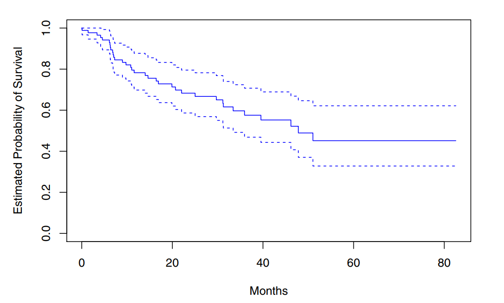
Each point in the solid step-like curve shows the estimated probability past the time indicated on the horizontel axis, the estimated probability of surviving past 20 months is 71%.
The sequential construction of the Kaplan_Meier estimator (starting from time 0 and mapping out the observed events as they unfold in time) is fundemtal to many key techniques in survival analysis.
Conclusion
To conclude, Kaplan-Meier method is a clever method of statistical treatment of survival times which not only makes proper allowances for those observations that are censored, but also makes use of the information from these subjects up to the time when they are censored.
**Disclaimer: all the examples,derivations,numbers and charts are taken from the text book "An Introduction to Statistical Learning with Applications in R"**.