Linear Regression is one of the most important models in machine learning, it is also a very useful statistical method to understand the relation between two variables (X and Y).
Despite the apparent simplicity of Linear regression, it relies on several assumptions that should be validated before conducting a linear regression model.
- Linear Relationship: The response variable (Y) should be in a linear relation with the explanatory variables (X).
- Residuals Homoscedasticity : The residual errors should be of a constant variance at any value of X.
- Independence of Residuals : After fitting the linear regression model, residuals should be independent random variables.
- Normality of Residuals : The residual errors should be normally distributed.
Throughout the next lines, These assumptions will be explained, clarifying the significance of each, and how to be validated.
Linear Relationship
As you’ve chosen to conduct linear regression, then you are assuming that there is a linear relation between the explanatory variable (X) and the response variable (Y), following the below general equation :
Y = β*X + ϵ
Y : The response Variable.
X : The explanatory Variable.
β : The Linear Regression Coefficients.
ϵ : The Residual error Term.
There are two ways to validate this assumption:
- Drawing a scatter plot between each of the explanatory variables (X) and the response variable (Y), and then visually check the degree of the linear relationship between them.
- Checking of Pearson Correlation between each of the explanatory variables and the response variable, and to get a quantitative feel of the degree of linearity between them.
Important Note: Pearson Correlation is a statistical test used to check the degree of linearity.
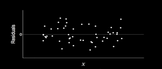
Residuals Homoscedasticity
Residuals Homoscedasticity refers to a condition in which the variance of the residuals/error terms is constant.
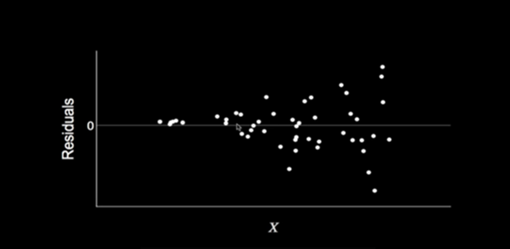
The property of the data set to have a constant variance is called homoscedasticity, and its opposite, where the variance varies with the explanatory variable X is called heteroscedasticity.
Using Runs Test for Randomness
It is a statistical test used to determine if the data obtained from a sample is random or not. The Run simply indicates the number of switches between events (A certain event followed by a different event is called a run). To be able to perform the run test on residuals we will do the following steps :
At the presence of heteroscedasticity residuals are a function of the explanatory variables and they will vary depending on them, so the residuals are not independent of the explanatory variables anymore!
Besides that heteroscedasticity makes the model’s predictions uninterpretable, Recalling that ordinary least-squares (OLS) regression seeks to minimize residuals and in turn produces the smallest possible standard errors. OLS regression gives equal weight to all observations, but when heteroscedasticity is present, this method is no longer valid, as a result we can easily suspect the validity of the regression model weights.
What are the possible reasons for heteroscedasticity?
1.Data Outliers: observations that are either small or large with respect to the other observations are present in the sample.
2.The omission of variables from the model: When you Omit a relevant variable out of a model, the omitted effect is absorbed into the error term. If the effect of the omitted variable varies throughout the observed range of data, it can produce heteroscedasticity in the residual plots.
How can we detect the presence of heteroscedasticity?
There are several ways to detect heteroskedasticity, but the most common is The White Test .
As stated, the linear regression equation can be described by the following equation: Y = β*X + ϵ
Where ‘ϵ’ represents the residual errors and ‘X’ represents the explanatory variables.
So, we need to make sure that there is no relation between ‘ϵ’ and ‘X’, to do so we will describe a new relation which is the Auxiliary Regression relation
𝜖²=𝛾 (0) +𝛾 (1) 𝑋1+……+𝛾(𝑛)𝑋𝑛+𝛾(𝑛+1) 𝑋¹²+……+𝛾(2𝑛)𝑋𝑛²+𝛾(2𝑛+1)𝑋1𝑋2+…….
To be able to prove homoscedasticity, we need to prove that there is no relation between the residuals (𝜖) and explanatory variables X and their squares (X²) and cross-products (X X X).
So, we need to prove that all the coefficients of explanatory variables X and their squares (X²) and cross-products (X X X) are exactly equal to 0.
We are striving to end up with the following equation: 𝜖2=𝛾 (0).
But, the above equation is really so complicated, and it introduces a lot of constraints on the regression coefficients, that’s why a nicer equation came up introducing the same concept but with much less terms.
𝜖2=(0) +𝛼(1)𝑌+𝛼(2)𝑌²
If we are able to prove that 𝛼 (1) and 𝛼 (2) are of ‘0’ values , then we will be able to prove that their no relation between the residual error (𝜖) and the predicted variable (Y) , then implicitly there is no relation between the residual error (𝜖) and the explanatory variable(X) .
We will estimate the coefficients (1) and 𝛼(2) using OLS Model , Then F-Static test is used to determine the significance of the coefficients , if the F-Test returns a P-Value > 0.05 then we can accept the null hypothesis (𝛼 (1) = 𝛼 (2) =0 ) , and then we will have enough evidence that there is no meaningful relation between the residual errors and the predicted variable.
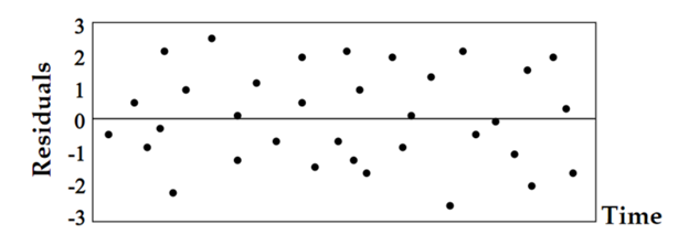
Independence of Residuals
This Assumption indicates that there should not be dependency between the residuals.
So, the current value of residual error is totally independent on the previous/historic values, just like rolling a die twice, the probability of getting ‘1’ the first time is totally independent on the probability of getting ‘1’ the second time.
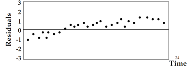
If the residual errors are dependent, they will likely produce a clear pattern, which indicates that there are information that the regression model did not capture and this information turned out to be a residual error, making our model sub-optimal.
How to test for independence of residual errors?
There are common techniques to detect the dependence of residuals, we will state two of them:
Using Runs Test for Randomness
It is a statistical test used to determine if the data obtained from a sample is random or not. The Run simply indicates the number of switches between events (A certain event followed by a different event is called a run). To be able to perform the run test on residuals we will do the following steps :
1. Define the null and alternative hypothesis
Null hypothesis: the residuals errors are random.
Alternative hypothesis: the residual errors are dependent.
2. Put the residual errors as a series of numbers in order of occurrence.
Example:
18- 36- 19- 22- 25- 44- 23- 25- 27- 35
3. Get the median of the residual errors.
Median: 25
4. Label any residual error less than or equal to the median with A and any residual error more than the median with B.
18(A)- 36(B)- 19(A)- 22(A)- 25(A)- 44(B)- 23(A)- 25(A)- 27(B)- 35(B)
5.Determine the number of runs and the number of each kind of events.
A — B — AAA — B — AA — BB
R=6 , n(B)=4 , n(A)=6
6.Using n(A) and n(B), we can use the statistical tables to get the critical values .
Upper critical value:2 and Lower critical value:9
Since R is between the critical values, so we have enough evidence to accept the null hypothesis.
Using Dubin-Watson test
It which measures the degree of correlation of each residual error with the ‘previous’ residual error. This is known as lag-1 auto-correlation. The Durbin Watson test reports a test statistic, with a value from 0 to 4, where:
2 is no auto-correlation.
0 to <2 is positive auto-correlation.
$\gt$2 to 4 is negative auto-correlation.
Normality of Residuals
In this section we will introduce a new constraint to the residual errors, residual errors should be normally distributed with a mean of 0 and constant standard deviation.
Normality is telling you implicitly that most of the residual errors are around the mean which is 0.
What if residuals are not following a normal distribution?
If the residual errors of regression are not normally distributed, then we cannot trust the coefficients of the linear regression model.
Because simply the tests used that are used to determine the significance of the model’s coefficients are valid only under the assumption of the normality of residual errors, such as F-Test for regression analysis .
But its important to state that violation of the normality assumption only becomes an issue with small sample sizes, as for the large sample sizes the assumption is less important due to the central limit theorem.
How to detect the normality of the residual errors?
There are a lot of ways to test for the normality of residual errors, and even though normality can be checked visually by drawing a histogram of the residual errors and check the shape of the distribution, we prefer to use static tests to detect the degree of normality if residual errors such as:
-
Shapiro-Wilk test: simply it quantifies the similarity between the residual errors distribution and a perfect normal distribution, by superimposing a normal curve over the distribution of the residual errors, then computing the percentage of samples overlap “Similarity Percentage”
-
Jarque-Bera test: it’s usually used for large sample size, The test matches the skewness and kurtosis of the data to see if it matches a normal distribution, noting that a perfect normal distribution has a mean of value ‘0’ and kurtosis of value ‘3’.
- Skewness tells us how symmetric the distribution is (Is it pulled to the right or the left)
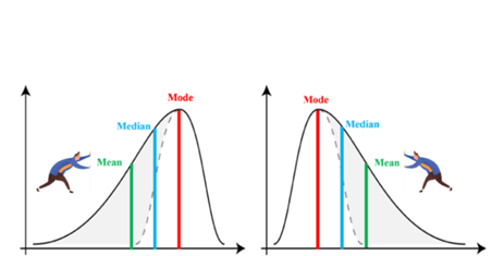
- Skewness tells us how symmetric the distribution is (Is it pulled to the right or the left)
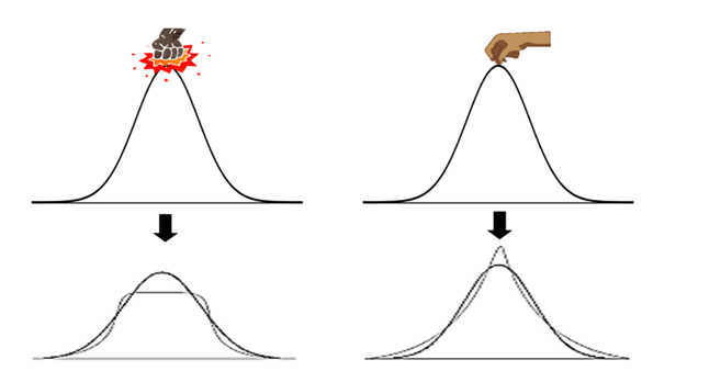
- Kurtosis tells us information about the peak and the tail of the curve (think about punching or pulling the normal distribution curve from the top).
Summary
The Linear Regression model is immensely powerful and a long-established statistical procedure, however, it’s based on foundational assumptions that should be met to rely on the results.
Good knowledge of these assumptions is crucial to create and improve the model.
When building your linear regression model, it is important to verify that the assumptions are respected and to tackle any potential violations in case they arise.